EPM AI – Advanced Prediction – From Setup to Strategy – Part2

Posted by Jun on September 8, 2025October 12, 2025

Part 2 – Algorithms, Model Logic & Interpretation, and Real‑World Use Cases

🔗 Read the Full Series

Introduction

In Part 1, you learned how to build the scaffolding of an Advanced Prediction model. Now, we dive deeper, exploring the algorithm engine, interpretation techniques, and how to adapt the model for real-world business use.

This part is data science adjacent territory, and I’ll explain what’s happening under the hood and how to use outputs in your planning process.

1. The Algorithm Landscape & AutoMLx

Advanced Predictions support a range of ML and statistical algorithms, from simple exponential smoothing to ensemble ML models.

Oracle’s Advanced Predictions supports and leverages a robust portfolio of modeling techniques. You can choose a subset manually or let AutoMLx run them all and pick the best.

Supported Algorithms

Oracle AutoMLx

NaiveForecaster – Naive and Seasonal Naive method
ThetaForecaster – Equivalent to Simple Exponential Smoothing (SES) with drift
ExpSmoothForecaster – Holt-Winters’ damped method
STLwESForecaster – Seasonal Trend LOESS (locally weighted smoothing) with Exponential Smoothing substructure
STLwARIMAForecaster – Seasonal Trend LOESS (locally weighted smoothing) with ARIMA substructure
SARIMAXForecaster – Seasonal Autoregressive Integrated Moving Average
ETSForecaster – Error, Trend, Seasonality (ETS) state space Exponential Smoothing
Prophet Forecaster – Facebook Prophet, only available when explicitly provided to the AutoML Pipeline through the model list parameter.
ExtraTreesForecaster – A reduction-based machine learning model based on ExtraTrees regression model
LGBMForecaster – A reduction-based machine learning model based on LGBM regression model
XGBForecaster – A reduction-based machine learning model based on XGB regression model

2. Under the Hood: Model Fitting, Validation & Overfitting Guardrails

When AutoMLx trains models, here’s roughly what happens:

Train/Validation Split: The historical window is segmented (e.g., 80/20 split or rolling folds)
Feature Transformations: Some models require stationarity or detrending; others implicitly manage that
Hyperparameter Search: For ML models (e.g. XGBoost, LightGBM), a grid or random search is done (within bounds)
Residual Analysis: After training, residuals (actual – fitted) are analyzed for bias, heteroscedasticity, autocorrelation
Model Selection: The algorithm with minimal error and acceptable residual behavior is chosen
Confidence Interval Estimation: Many models (especially statistical ones) naturally generate error bounds; for tree-based models, quantile regression or bootstrapping may be used

This “trial by algorithm” approach spares you from manual hyperparameter tuning while still giving flexibility to override when needed.

Oracle’s internal pipeline wraps and abstracts this, so you don’t need to code it yourself, but the logic matters when interpreting output.

3. Interpretation – Turning Output into Business Insight

The raw numbers are useful, but the real value is in interpreting and explaining to stakeholders.

Fitted vs Actuals

Plot historical actuals along with the fitted values line. Where they diverge, you can see which periods your model “missed” (e.g. shocks, structural breaks).

Residual Analysis & Diagnostics

Check residual plots (error over time) for patterns (bias, autocorrelation). If residuals are not white noise, it suggests model misspecification.

Feature Importance / Driver Contribution

While explainability is on the roadmap, you can already see which drivers contributed most (in ML models). This is critical to trust: e.g., “Promotions explain 30% of variance, GDP 15%, base trend 55%.”

Event Impact Overlay

When you enable events (recurring / one-off), the model can overlay the event’s effect. You can visually see how events pushed deviation vs baseline.

Confidence Bands

Use P10–P90 bands to guide risk assessment. For example:

If a forecast’s lower bound is still above the desired threshold, the target is safe.
If the band is wide in volatile periods, you may want conservative planning.

Version Comparison

Because Oracle allows you to save results per algorithm version, you can run multiple configurations (e.g. AutoMLx vs XGBoost) and allow planners to switch on forms to see alternative predictions side-by-side.

4. Expanded Use Cases

Use Case A: Product Revenue Forecasting

Target: Monthly revenue

Drivers:
– Promotions (dollar spend)
– Average selling price
– Industry index (macro)
– Holiday season dummy

Approach:
– Run baseline with 2 drivers (promo, price)
– Expand to 4–5 drivers
– Compare error vs univariate model

Insight: Model may show that promotions drive 25–30% of variance; price elasticity is captured more dynamically.

Use Case B: Workforce Planning & Attrition

Target: Headcount / attrition

Drivers:
– Average tenure
– Age distribution
– Satisfaction scores
– External unemployment rate

Value: You can simulate a shift in satisfaction and estimate downstream attrition, enabling proactive recruiting or retention policies.

Use Case C: Service / Product Hybrid Model

Target: Call volume, service headcount, cost

Drivers:
– Number of product units in field
– IoT usage metrics (hours in service)
– Incident rates
– Maintenance schedules

Value: As you shift from sale to “service as a product,” you can forecast the resource plug-in impact.

Use Case D: Event-Sensitive Sales Forecast

Events: Product launches, promotions, supply chain disruptions, holidays

Approach: Label events as recurring fixed (e.g. Christmas), recurring movable (e.g. Ramadan), one-off (e.g. plant outage), or skip (pandemic).

Benefit: Enables pre- and post-event planning sensitivity analyses, i.e. “if Olympic demand surges, how does the forecast shift?”

5. Challenges, Limitations & Workarounds

Limited explainability today (feature importance is roadmap)
Overfitting risk with many drivers and small historical window
Missing/faulty driver data can degrade models
Event representation complexity: misclassifying events can mislead forecasts
Processing latency for large models
Parent-level prediction limitations (until dynamic calc roadmap)

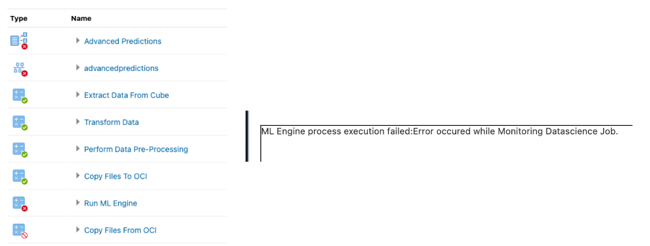
Also, when running the model, sometimes it gets stuck on the OCI data science job.

Workarounds:

Regularly backtest and monitor performance
Keep driver counts modest initially
Use domain logic to vet feature importance
Use rolling-origin splits in backtesting
Use simple models in volatile domains

Conclusion & What’s Next

By now, you should understand not only what the engine runs but why and how to interpret its outputs meaningfully for planning.

In Part 3, we’ll focus on long-term strategy: feature engineering roadmap, dynamic parent-level prediction, deployment best practices, and how to embed Advanced Prediction into your FP&A operations.